-
 contact@diggers-consulting.com
  01 73 28 29 65
 LinkedIn


When we talk about machine learning in finance, we often imagine complex models predicting market movements or flagging suspicious trades. In reality, even relatively simple algorithms can reveal fascinating insights. In this article, I’ll show how two very different machine learning models — an AutoEncoder (a type of neural network) and a Gaussian Process (a probabilistic model) — can detect anomalies in stock prices, using the famous case of GameStop (GME) during 2020–2021.
A Bit of Context: What Happened with GME?
At the start of 2021, GameStop’s stock experienced one of the most dramatic short squeezes in modern financial history. Driven by retail investors on Reddit, GME’s price skyrocketed from around $20 in early January to nearly $500 within weeks — then crashed just as fast.
This extreme volatility makes GME a perfect test case for anomaly detection: any model that tries to understand the “normal” behavior of the stock should be completely confused when the squeeze happens. That’s exactly what we want to measure.
Machine Learning Families: Where These Models Belong?
Before diving into results, it’s helpful to understand where each model fits in the machine learning ecosystem.
AutoEncoder (AE):
Part of the neural network family, AutoEncoders are designed to learn patterns by compressing and reconstructing data. They don’t predict the future directly but instead learn what “normal” looks like. When the model can’t reconstruct an input accurately, it likely encountered something unusual — an anomaly.
Gaussian Process (GP):
A probabilistic, non-parametric Bayesian model: “non-parametric” means it doesn’t assume a fixed number of parameters and can adapt its complexity to the data; “Bayesian” means it treats predictions as distributions, capturing uncertainty rather than giving a single fixed value. It adapts the initial distribution once it has observed data.
It doesn’t have neurons or layers. Instead, it assumes every point in the dataset belongs to a smooth function and models the relationships between all points. These relationships are captured using a kernel (or covariance) function, which measures the similarity between points: points that are more similar have more strongly correlated outputs. A GP predicts both the expected value and the uncertainty of that prediction — perfect for identifying points that fall far outside normal confidence bounds.
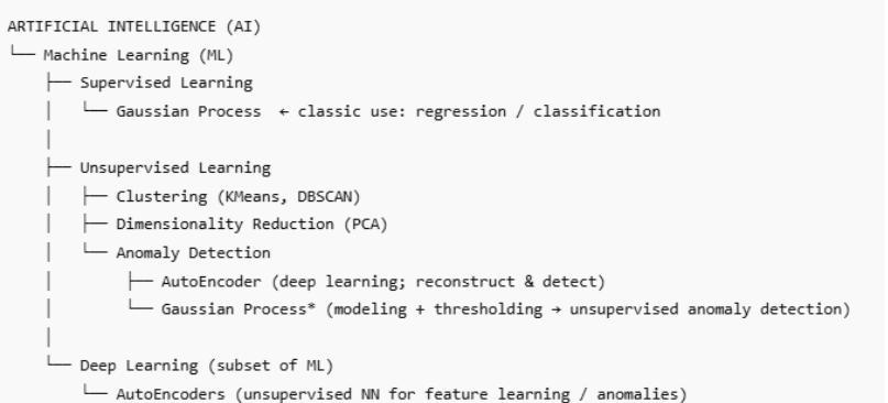
Here is a quick overview of the ML ecosystem and our models’ placements in it:
How the Models Were Applied and first results
I trained the AutoEncoder on GME closing prices from 2020 and tested it on 2021 data. The model looked at 10-day sliding windows of prices and tried to reconstruct them. When the reconstruction error (residual) was too high — both in absolute and relative terms — I flagged that period as an anomaly.
For the Gaussian Process, I used an RBF (Radial Basis Function) kernel, most common one, which enforces smoothness. The GP fit the entire time series and produced a predicted mean and standard deviation for each day. When the real price deviated beyond two standard deviations and more than 10% from the mean, that day was marked as an anomaly.
First results:
Unsurprisingly, both models were triggered around January 2021 — the period of the massive short squeeze. But there were interesting differences:
The AutoEncoder was highly sensitive to local, short-term changes. It picked up not only the main squeeze but also smaller aftershocks — price rebounds and corrections.
The Gaussian Process reacted more conservatively. Because it assumes smoothness, it smoothed over sharp jumps and identified broader deviations from long-term trends rather than daily spikes.
When compared, some anomalies overlapped (clear market shocks), while others were unique to each model — showing that the two methods capture different types of irregularity.
Gaussian Process vs Neural Network: Two Different Minds
Although both methods are used in machine learning, they represent completely different philosophies.
- An AutoEncoder is neural: it learns a single function by adjusting weights through many layers.
- A Gaussian Process is Bayesian: it assumes all possible functions and finds the most likely one given the data.
Together, these models can complement each other: the GP gives a stable macro view, while the AutoEncoder detects micro shocks.
AutoEncoder — Strengths and Limits
- Strength: Great at capturing short-term volatility.
- Limit :Sensitive to scaling and window size. If the window is too short, it misses patterns; if too long – it smooths them out.
- Improvement: Try with LSTM (Long Short-Term Memory) AutoEncoders and adaptive thresholds based on volatility.
Gaussian Process — Strengths and Limits
- Strength: Naturally provides uncertainty estimates — very useful in finance.
- Limit : Assumes smoothness, which fails during extreme events like the GME squeeze.
- Improvement: Use non-stationary kernels where for every point not only neighbour points count, but the whole data series or mixtures of kernels (RBF + WhiteKernel) to adapt to changing volatility and jumps.
Going Further
The GME case is a perfect reminder that markets are anything but smooth. No model can predict a social-media-fueled trading storm — but models can help us see when something unusual happens.
This article is just the beginning. If you’d like to go further, try:
- Replacing the dense AutoEncoder with an LSTM AutoEncoder for temporal awareness.
- Play with different kernels to adapt uncertainty dynamically.
If you want to apply the same logic to other events — like the 2008 crisis or the 2010 Flash Crash — to see how anomalies evolve across different regimes feel free to use my code.
Python: How the Code Works
You can easily adapt my Python code for other stocks and time periods.
These are the libraries that I used: numpy, matplotlib.pyplot, yfinance, sklearn.preprocessing, tensorflow.keras.models,tensorflow.keras.layers,sklearn.gaussian_process,klearn.gaussian_process.kernels. You will find details in “requirements.txt”.
And here comes a quick breakdown:
- Data Download: The script fetches stock price data from Yahoo Finance using the yfinance library.
- AutoEncoder Setup: The data is scaled with StandardScaler, split into overlapping 10-day windows, and fed into a simple neural network built with Keras. The network tries to reconstruct its own input. Large reconstruction errors are flagged as anomalies.
- Parameters like ae_window_size, ae_epochs, and thr_abs_ae control how sensitive the detection is.
- Gaussian Process Setup: A Gaussian Process model is built using scikit-learn with an RBF kernel. It fits the full price curve, predicts both mean and uncertainty, and marks anomalies where deviations exceed the expected range.
- gp_alpha adjusts noise sensitivity, while thr_pct_gp defines how large a deviation must be to be considered unusual.
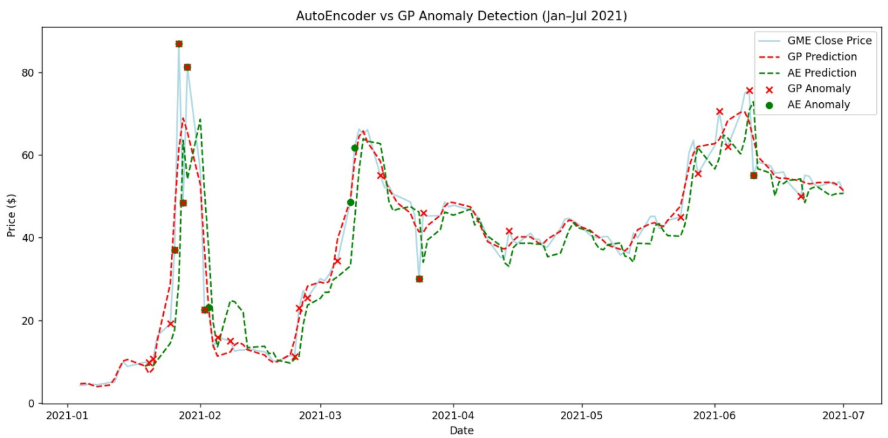
- Comparison and Visualization: The final part of the script aligns anomalies detected by both models and plots them against real GME prices between January and July 2021.
- Green points show AutoEncoder anomalies, red crosses mark Gaussian Process anomalies.
- Overlaps highlight where both models agree — the strongest anomaly signals.
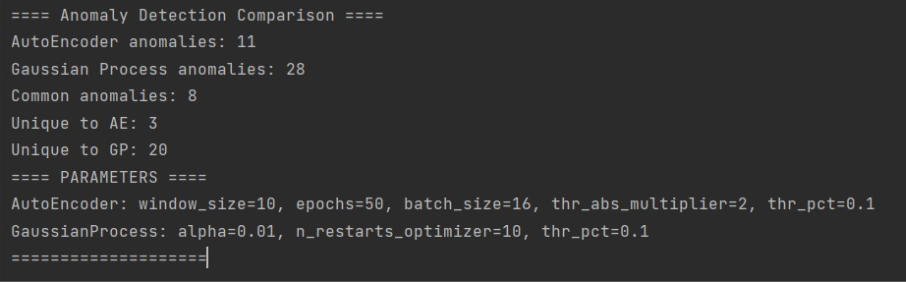
- Running the script will print summary statistics (how many anomalies were detected, how many overlapped, etc.) and display a chart comparing both methods.
Bonus – Parameters to plays with: The good entry point is to play with basic parameters, trying to avoid common AI problems like lack of training or overfitting.
- Thresholds: Both models can use std or % thresholds depending on your implementation.
- AE Epochs / Batch: Longer epochs = better learning but risk of overfitting. Batch size affects stability.
- GP Alpha: Controls noise; higher → smoother predictions, lower → more sensitive to anomalies.
| Model | Parameter | Current | Values to Test |
| AutoEncoder | Threshold (std) | 2 | 1.5, 2, 2.5, 3 |
| AutoEncoder | Threshold (%) | 1 | 0.5, 1, 2, 5 |
| AutoEncoder | Epochs | 100 | 50, 100, 150, 200 |
| AutoEncoder | Batch size | 64 | 32, 64, 128 |
| GP | Threshold (std) | 2 | 1.5, 2, 2.5, 3 |
| GP | Threshold (%) | 1 | 0.5, 1, 2, 5 |
| GP | Alpha | 1e-5 | 1e-5, 1e-4, 1e-3, 1e-2 |
Good luck!