What is a Deep Neural Network and why to use it?

Each layer in DNN extracts and learns abstract features from the data, allowing the network to make more complex and accurate predictions or decisions. This process of learning from data is known as training the network and involves adjusting the weights of the connections between neurons.

DNNs are widely used in image and speech recognition, natural language processing, and self-driving cars. Today we will use DNN to price an option.

Major types of DNN

There are several types of deep neural networks, each designed for specific tasks and architectures. For example, Convolutional Neural Networks (CNNs) – are primarily used for image and video recognition. They consist of multiple convolutional layers that apply filters to the input data, allowing the network to learn spatial features and patterns.

Another good example to learn is a Physics-Informed Neural Network (PINN). This type of DNN is designed to solve partial differential equations (like Black-Scholes or Navier-Stokes).

Here, we will focus on the easiest and most intuitive DNN which is a Feedforward Neural Network (FNN). An FNN consists of an input layer, one or more hidden layers, and an output layer. The input layer would take the parameters of the option (e.g. stock price, strike price, time to maturity) as input, and the output layer provides the estimated price of the option as output. The hidden layers would contain neurons that apply nonlinear transformations to the input data, allowing the network to learn complex relationships between the input variables and the option price.

Here is a simple representation of a FNN:

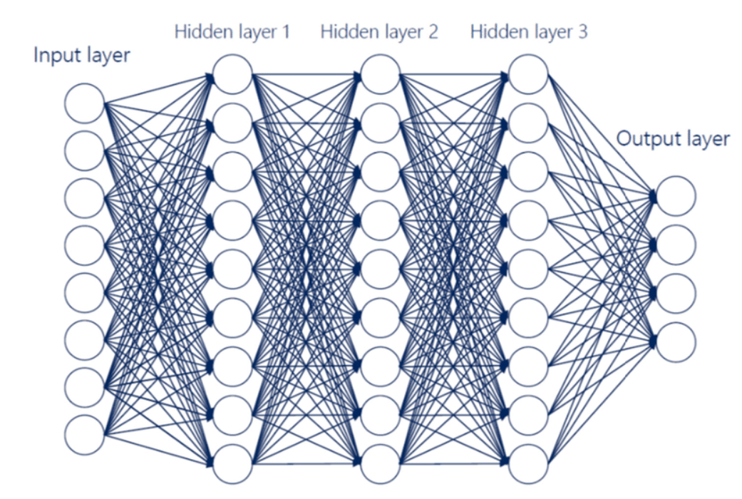
As you can see, each node (or neuron) in the layer is connected to every node in the previous layer. This type of layer is called a Dense layer.

In addition to dense layers, there are many other types of layers that can be used in DNN: Convolutional Layers, Pooling Layers, Recurrent Layers, Dropout Layers, and so on. But today we will focus on the DNN of type FNN with 3 dense layers.

Creating a DNN with Python

Firstly, we would like to share the most commonly used Python libraries that allow you to create a DNN:

1. TensorFlow – the most popular one
2. PyTorch – mostly used for PINN to solve PDE
3. Keras – the one we use here to price an option

In order to create a DNN to solve the Black-Scholes Partial Differential Equation (PDE), we will take the following steps:

1. Define the problem: First, the problem needs to be defined, which involves identifying the inputs (e.g. stock price, strike price, time to maturity, volatility), the output (option price), and the governing equation (the Black-Scholes PDE)
2. Design the DNN: The DNN architecture needs to be designed, which involves choosing the number and type of layers, the number of neurons in each layer, and the activation function to be used.
3. Train the DNN: The DNN needs to be trained on the prepared dataset using a suitable optimization algorithm, such as stochastic gradient descent (SGD) or Adam. During training, the network adjusts its parameters to minimize the difference between the predicted option prices and the true option prices from the dataset.
4. Use the DNN for prediction: Once the DNN has been trained and evaluated, it can be used for predicting option prices for new input data.

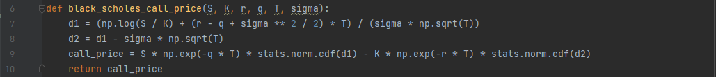
First of all, we create a governing equation:

Then we need to create a method that will define our DNN and train it:

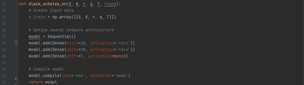
As it was mentioned before, we are using Keros library. Let’s go through the classes used here.

Sequential() - is a class in the Keras that allows you to build a sequential model in a linear stack of layers. In other words, you can create a model by adding layers to it one by one, in a sequential manner. It fits perfectly our goal, which is a FNN.

model.add(Dense(units=10, activation='relu')) - add method adds a new layer, but we have to define it. We need a Dense layer of 10 units, where units being the number of neurons or nodes in a particular layer. Every layer can have different number of units and it can be seen as the weight matrix that connects the layer to the previous layer. The activation is an optional argument that specifies the activation function to be used in the layer. It takes several values - Sigmoid, Softmax, etc. We use ReLU as it's one of the most commonly used activation functions in deep learning due to its simplicity and efficiency. In the last line, the value None is used, which means that the layer will produce a linear output without applying any non-linearity.

model.compile(loss='mse', optimizer='adam') - this function take 2 arguments. The first one - loss -specifies the loss function that will be used to evaluate the performance of the model during training. In this case, the 'mse'  stands for Mean Squared Error. The optimizer specifies the optimizer algorithm used to update the weights of the model during training. The algorithm adam is the most popular one.

model.fit(x_train, np.array([black_scholes_call_price(S, K, r, q, T, sigma)]), epochs=200, batch_size=256, verbose=0) - the fit method is used for training our model, its takes several arguments:
 - x_train: This is the input data used for training the model. In this case, it is assumed to be the input variables used to calculate the Black-Scholes call option price, such as the stock price S, strike price K, risk-free interest rate r, dividend yield q, time to expiration T, and volatility sigma.
 - np.array([black_scholes_call_price(S, K, r, q, T, sigma)]): This is the target output value used for training the model. It is assumed to be the Black-Scholes call option price calculated using the input variables S, K, r, q, T, and sigma. The black_scholes_call_price function defined earlier is called to calculate this value.
 - epochs=200: This specifies the number of times the model will iterate over the entire training dataset during the training process.
 - batch_size=256: This specifies the number of samples that will be used in each batch during the training process.
 - verbose=0: This specifies the verbosity level during training. If set to 0, no output will be printed during training. You may try verbose=1 - it then will output a progress bar for each epoch of training, showing the current epoch number, the total number of epochs, and the training loss at the end of each epoch.

The core of ou DNN is built. Once we have defined S, K, r, q, T, and sigma, we need to create a big training set and to train our model:

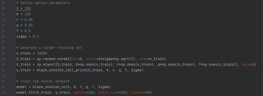
The crucial part of applying a DNN is a training process. The larger the training set and the number of itiration - the more accurate is the final result. Let's take a closer look at fit() method:

model.fit(X_train, y_train, epochs=200, batch_size=256, verbose=0) - the fit method is used for training our model, its takes several arguments: 
- X_train: This is the input data used for training the model. In this case, it is assumed to be the input variables used to calculate the Black-Scholes call option price, such as the stock price S, strike price K, risk-free interest rate r, dividend yield q, time to expiration T, and volatility sigma.  
- y_train:  This is the target output value used for training the model. It is assumed to be the Black-Scholes call option price calculated using the input variables S, K, r, q, T, and sigma. 
- epochs=200: This specifies the number of times the model will iterate over the entire training dataset during the training process. 
 - batch_size=256: This specifies the number of samples that will be used in each batch during the training process. 
 - verbose=0: This specifies the verbosity level during training. If set to 0, no output will be printed during training. You may try verbose=1 - it then will output a progress bar for each epoch of training, showing the current epoch number, the total number of epochs, and the training loss at the end of each epoch.

Now, our model is trained. Let’s try to run it with another value of S and compare it to the results of the function black_scholes_call_price. Note, that we use predict() method here:

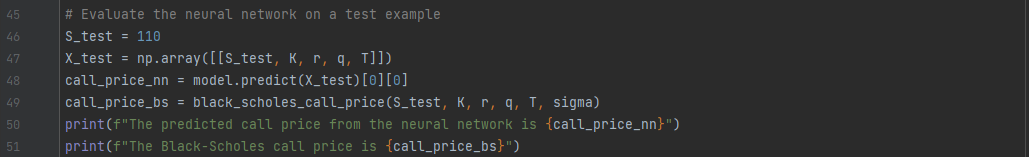
So, the output is:

which is pretty close and varies at every run as the DNN is a learning mechanism first of all.

Let’s do another run but this time with model.fit(X_train, y_train, epochs=2, batch_size=256, verbose=0):

This time the result is less accurate as the model was not enough trained.

DNN is a very promising tool that has already shown its efficiency in many fields. Basic knowledge of this concept is crucial for those who are interested in option pricing. The model we used here is quite basic, the next step might be using PINN instead of FNN.

Here you can find the full code of this example.

Article précédent

Article suivant