What is FFT and why use it in Option pricing?

FFT stands for Fast Fourier Transform.

The FFT has numerous applications in digital image processing, audio compression, and finance.

For example, FFT allows analysis of data series: it can reduce the noise or find periodic data patterns, but in this article, we will focus on FFT in Option Pricing.

Typically, Option Pricing models have no closed-form analytical solution with few exceptions (Black-Scholes, CRR, Bates models). But we can overcome it with Monte-Carlo Simulation or Finite Element Method. FFT is just one more technique that allows us to price an option regardless of its type.

How to price an option with FFT

Before we compare the main FFT algorithms, let’s take a look at the major steps of applying those FFT algorithms in Option Pricing.

The main idea behind the Fourier method is to use the characteristic function of the underlying asset price to calculate the option price.

The underlying asset price can follow any Lévy process, alone or combined: Wiener process, Poisson + Wiener process, Normal Inverse Gaussian process, etc.

The characteristic function is a strong mathematical concept – it completely defines the probability distribution of a random variable. And if the random variable admits a probability density function, then the characteristic function is the inverse Fourier transform of the probability density function. Thus, the characteristic function is usually well-known or can be easily derived from the probability density function.

Pricing options using the FFT method involve the following steps:

1. Collect the necessary market data (current market price of the underlying asset, the option’s strike price, time to expiration, etc)
2. Select a suitable pricing model or process (Black-Scholes, Compounded Poisson, Heston, etc)
3. Find the option’s characteristic function regarding the chosen model or process
4. Apply the FFT algorithm to a resulting integral:
   1. Choose the FFT algorithm
   2. Apply the chosen FFT algorithm to evaluate the integral that computes the option price
5. Compute the option price (use the output of the FFT algorithm to compute the option price)

Even though this technique is quite simple, it deserves a separate article. But today, we will pay attention to 4.1.

What are different FFT algorithms?

There are several algorithms for computing the FFT, each with its own advantages and disadvantages even though nominally, they have the same complexity O(N log N). The most commonly used algorithms for computing the FFT are:

1. Cooley-Tukey Algorithm
2. Radix-2 FFT Algorithm
3. Bluestein’s Algorithm
4. Prime Factor Algorithm

Let’s take a closer look at each one of them and then compare the complexity.

The Cooley-Tukey algorithm

The Cooley-Tukey algorithm is a widely used algorithm for computing the FFT of a sequence. The algorithm is based on the divide-and-conquer approach, which involves breaking the input sequence into smaller subsequences and recursively computing the FFT of each subsequence.

The Cooley-Tukey algorithm works by dividing the input sequence of length N into two subsequences of length N/2. The FFT of each subsequence is then computed recursively using the same algorithm. After computing the FFT of the two subsequences, the results are combined to produce the final FFT of the input sequence.

The key to the Cooley-Tukey algorithm is the fact that the DFT of an N-point sequence can be computed using the DFTs of two N/2-point sequences. Specifically, let x(n) be an N-point sequence, and let X(k) be its DFT. Then, the DFT of x(n) can be expressed as:

where E(k) and O(k) are the DFTs of the even and odd-indexed elements of x(n), respectively, and W_N^k is the twiddle factor, defined as:

for k = 0, 1, …, N-1.

The Cooley-Tukey algorithm takes advantage of this property by computing the DFT of the even-indexed elements and the odd-indexed elements separately and then combining them using the twiddle factors.

The Radix-2 FFT Algorithm

The Radix-2 FFT algorithm is a fast algorithm for computing the FFT of a sequence of length N that is a power of 2 (i.e., N = 2^k). It is based on the Cooley-Tukey algorithm, which recursively divides the input sequence into smaller subsequences and computes their FFTs. However, the Radix-2 FFT algorithm uses a more efficient approach for dividing the sequence into even and odd-indexed subsequences.

The key idea behind the Radix-2 FFT algorithm is to use the fact that a sequence of length N can be divided into two subsequences of length N/2 by separating the even-indexed and odd-indexed elements of the sequence. Specifically, the Radix-2 FFT algorithm works as follows:

1. If the length of the input sequence is 1, return the input sequence as the output.
2. Otherwise, split the input sequence into two subsequences: one containing the even-indexed elements and the other containing the odd-indexed elements.
3. Recursively compute the FFTs of the two subsequences using the Radix-2 FFT algorithm.
4. Combine the two FFTs by multiplying the odd-indexed FFT by a sequence of « twiddle factors, » which are defined as W_N^k = exp(-j 2π k/N) where N is the length of the input sequence and k is the index of the element being computed.
5. The combined FFT is then given by concatenating the sum of the even-indexed FFT and the twiddle factors times the odd-indexed FFT with the difference of the even-indexed FFT and the twiddle factors times the odd-indexed FFT.

This algorithm is commonly used in software libraries for computing FFTs (i.e., Numpy in Python).

Bluestein’s algorithm

Bluestein’s algorithm is a fast algorithm for computing the discrete Fourier transform (DFT) of a sequence of arbitrary length N. It is based on the convolution theorem and works by transforming the input sequence into a new sequence of length 2N-1, which is then convolved with a carefully chosen « chirp » signal to obtain the DFT of the original sequence.

The key idea behind Bluestein’s algorithm is to use the convolution theorem, which states that the DFT of the convolution of two sequences is equal to the product of their DFTs. Specifically, the algorithm works as follows:

1. Pad the input sequence x with zeros to create a new sequence of length 2N-1.
2. Define a new sequence y of length 2N-1, where y[n] = x[n] * w[n], where w[n] is a « chirp » signal defined as: w[n] = exp(-j π n^2 / N)
3. Compute the DFT of the sequences x and y using the FFT algorithm.
4. Convolve the DFTs of x and y pointwise to obtain the DFT of the original sequence.

Bluestein’s algorithm has a time complexity of O(N log N), which is the same as the Radix-2 or Colley- Tukey FFT algorithms, but it is more computationally expensive due to the need to compute the chirp signal. It is most useful when the input sequence has a length that is not a power of 2 or when it is not sufficiently sparse.

The Prime Factor algorithm

The Prime Factor algorithm (PFA), also called the Good–Thomas algorithm, is an algorithm for computing the discrete Fourier transform (DFT) of a sequence of length N that is factorable into small prime factors.

Here are the steps of the PFA algorithm:

1. Factorize the length of the input sequence N into its prime factors. For example, if N=120, then its prime factors are 2, 2, 2, 3, and 5.
2. Rearrange the input sequence x[n] such that it is ordered according to a permutation of the original indices that groups together all of the indices that have a common prime factor. This can be accomplished using the Chinese Remainder Theorem (CRT). The result is a multi-dimensional array of size p1 x p2 x … x pk, where pi is a prime factor of N.
3. Compute the DFT along each dimension of the multi-dimensional array, starting with the dimension with the largest prime factor and working down to the dimension with the smallest prime factor. This can be done recursively by applying the PFA algorithm to each dimension one at a time.
4. Combine the intermediate results from each dimension using the CRT to obtain the final DFT of the input sequence.

The PFA algorithm is similar to the Cooley-Tukey FFT algorithm, but it is more general and can be used to compute the DFT of sequences with prime factors other than 2. It is also more efficient than the Cooley-Tukey FFT algorithm for sequences with a large number of small prime factors since it avoids the overhead of repeatedly shuffling the input sequence. However, for sequences with few prime factors, the Cooley-Tukey FFT algorithm is typically faster.

Key Differences

These 4 algorithms are all commonly used for computing the FFT of a data series (i.e., stock prices or signals). But here are some critical differences between them:

1. Data Length: The Cooley-Tukey algorithm and the Radix-2 algorithm are most efficient when the data length is a power of two. Bluestein’s FFT algorithm can handle arbitrary data lengths but is generally slower than the other algorithms. The prime factor algorithm is optimized for prime-length data series or data series that are the product of small primes.
2. Computational Complexity: The computational complexity of the Cooley-Tukey algorithm and the Radix-2 algorithm is O(N log N) for data series of N that is a power of two. The computational complexity of Bluestein’s FFT algorithm is also O(N log N), but with a larger constant factor than the other algorithms. The computational complexity of the Prime Factor algorithm is again – O(N log N).
3. Memory Usage: The Cooley-Tukey algorithm and the Radix-2 algorithm are both « in-place » algorithms, meaning that they compute the FFT of data series in the same memory space as the original signal. Bluestein’s FFT algorithm and the Prime Factor algorithm require additional memory to store intermediate results.
4. Implementation Difficulty: The Cooley-Tukey algorithm and the Radix-2 algorithm are both relatively easy to implement due to their recursive structure. Bluestein’s FFT algorithm is more complex to implement due to its use of convolutions. The Prime Factor algorithm requires more complex prime factorization techniques, which can make it more difficult to implement.

In summary, the choice of the FFT algorithm depends on the length of the data series (i.e., stock price) being processed. If the data length is a power of two, the Cooley-Tukey or Radix-2 algorithm may be the best choice due to its efficiency and ease of implementation. If the signal length is not a power of two or has other specific properties, Bluestein’s FFT algorithm or the Prime Factor algorithm may be more appropriate.

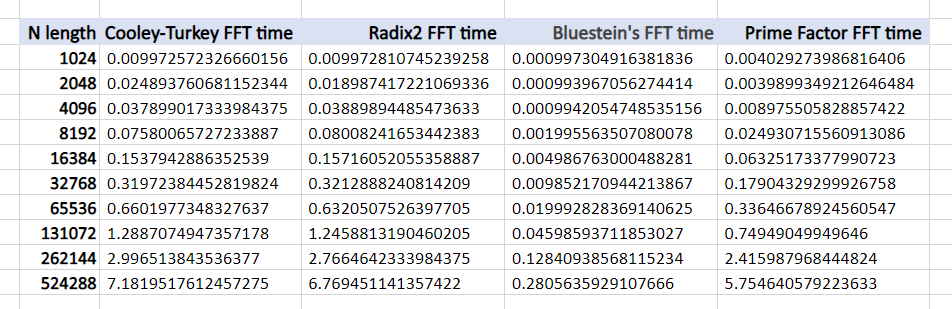
As it was mentioned before, today you can use the Monte-Carlo simulation or FEM method in Option pricing. The first one is quite expensive in memory, and the second one is very complex in implementation, so the FFT technique is a fair alternative but the key to success here is the choice of the right algorithm.

We have implemented these algorithms in Python and as you can see, the computation time changes drastically when N goes higher.

If you want to see the implementation in Python and test it yourself – find the code here.

If you want to find more on Option pricing with FFT – here is the paper that initially presented this method in 1998.

Article précédent

Article suivant