-
 contact@diggers-consulting.com
  01 73 28 29 65
 LinkedIn


Motivation
A model can be used for different purposes such as pricing or hedging for example. Pricing is the basis of Finance as every financial instrument needs to be continuously evaluated in order for an investor to approach the market with the best position possible. It is closely linked with the notion of hedging as a hedge is a move that is made with the intention of reducing the risk of adverse price movements in an asset.
Those articles are a genuine stepping stone to dive into the open-source library simultaneously developed. A library is a collection of prewritten methods that users can freely call. Thus, the main goal of this library is to provide functions to price several financial instruments in a generic fashion way. It will also help the reader to combine theory and practice by studying how those models can be implemented.
What derivatives will be priced ?
The term derivative refers to a type of financial contract whose value is dependent on several Risk factors such as a stock price, an interest rate, a volatility, a correlation, etc. It is set between two or more parties that can trade on an exchange or over the counter.
The initial purpose of this library is mainly to price Vanilla and Exotic options. A vanilla option is a financial instrument that gives the holder the right, but not the obligation, to buy or sell an underlying asset at a predetermined price within a given timeframe.
Both European-style and American-style options have been considered. A European-option specifies an expiration date. If the option is to be exercised, then the exercise must occur on the expiration date. On the other hand, an option whose owner can decide to exercise at any time up to the expiration date (included) is an American-option.
| Vanilla options | Call options (long or short position) and Put options (long or short position) |
| Exotic options | Asian options, Barrier options and Basket options |
| Fixed Income instruments | Zero-coupon bonds, Caps, Floors, Swaptions … |
Example of a European call option
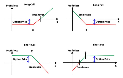
A European call option is an example of vanilla options. It can be described by the following payoff: (ST – K)+= max(ST – K,0), whereas a European put option is characterized by the following payoff: (K – ST)+.
Therefore, for a long position (meaning that the investor buys and owns the security) on a European call option, an investor expects the stock price at maturity, ST, to be above the strike price, K (+the call price) in order to make a profit and vice-versa for a long position on a European put option. Here is a recap of the payoff diagrams that can be encountered:
More details can also be found on the following link: https://www.investopedia.com/terms/c/calloption.asp.
According to Investopedia, Exotic options are a category of options contracts that differ from traditional options in their payment structures, expiration dates, and strike prices. The underlying asset or security can vary with exotic options allowing for more investment alternatives. Several Exotic options have been studied such as Asian options (with arithmetic and geometric means), Barrier options or Basket options. A recap about the payoff of these options can be found here: https://github.com/diggers-lab/DiggersPricers/blob/master/articles/payoff_Github.pdf.
Obviously, the library has been thought and structured in order to be able to price other derivatives such as Fixed Income instruments for instance. What is essential for a library is to be able to welcome changes without modifying its overall structure.
Structure of the library
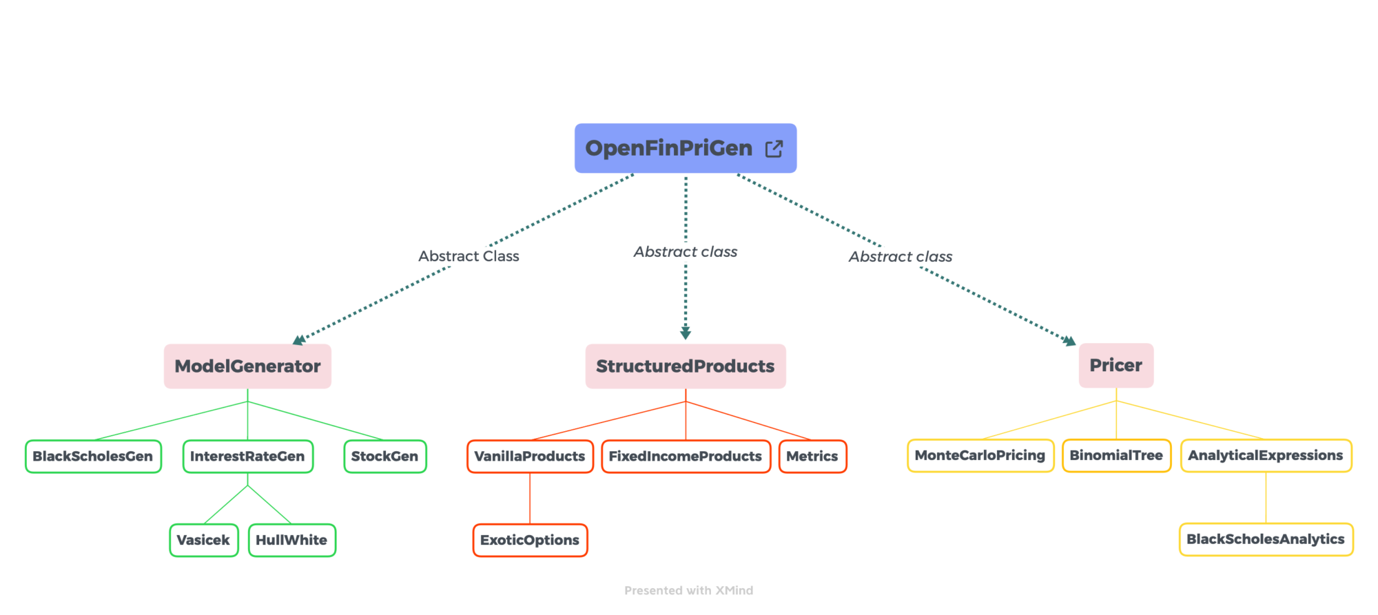
Our library is « OpenFinPriGen » and it is structured around three main abstract classes: ModelGenerator, StructuredProducts and Pricer.
First of all, ModelGenerator aims to generate every underlying asset according to a certain model. For example, it contains a subclass « InterestRateGen » that will provide different ways to simulate interest rates (Vasicek, Hull-White, etc). Stocks can also be modeled by different types of signals and random variables (GARCH, Geometric Brownian motion for example). The idea is to be able to stick to the dynamics imposed by a model and to simulate them thanks to a discretization.
Then, the abstract class StructuredProducts will provide the payoff of the derivative that needs to be priced. It is divided in different subclasses such as « VanillaProducts » (containing a subclass « ExoticOptions ») or « FixedIncomeProducts ». Some metrics can also be taken into account.
Finally, Pricer is a class containing different subclasses representing different techniques to price our products from a determined payoff. Among them, there is obviously « MonteCarloPricing » but also classes such as « BinomialTree » or « AnalyticalExpressions » as sometimes closed-form expressions exist to price certain derivatives.
Here is the Graph of the library:
Monte-Carlo Methods
Monte-Carlo methods are widely used in Finance for different reasons. Most of the pricing tests realized on this library have been realized thanks to these methods. The basis of a Monte Carlo simulation involves assigning multiple values to an uncertain variable to achieve multiple results and then averaging the results to obtain an estimate. It is quite a straightforward concept that mainly relies on the Law of Large numbers.
For example, to get the valuation of Interest Rate Derivatives, the idea is genuinely simple: generate a large number of equally probable rate paths, rn. Then, generate cash flows, CFn, along each path. Discount cash flows along each path as followed:
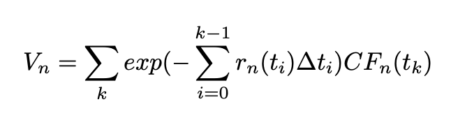
At last, take the average of the path values:
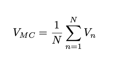
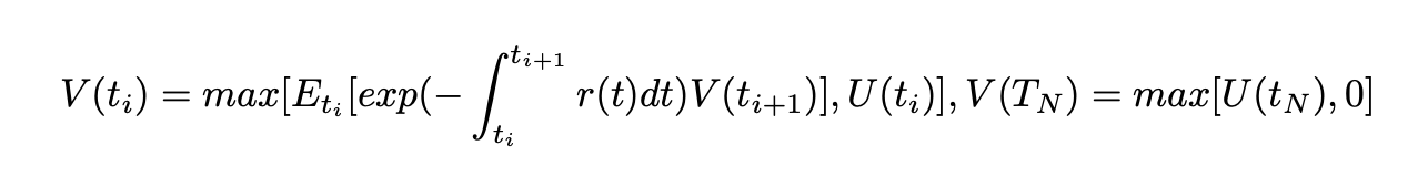
For an option with exercise times t1 <…< tN , and the exercise payoff function U(t), we have:
Admittedly, there are some limitations about Monte-Carlo Methods but they can be partially overcome and they will be discussed later.
Differences between models
A model provides dynamics about an underlying asset which means that it will follow certain properties and distributions according to assumptions imposed by the model. Usually, the main differences between models involve implied volatility (constant or not), interest rates (constant or not) and the underlying/asset (as the price evolves differently across asset classes).
What’s next ?
If you are interested and/or working in Finance/Quant Finance, you will find and rediscover some interesting topics. On the other hand, if you do not know anything about Finance, give it a try: you will understand more than you would actually think. Not everything is low-level nor high-level.
The next article will be about Black-Scholes-Merton model where spot interest rate is assumed to be constant as well as the volatility. It is the simplest model and the basic pillar of model pricing. Later, a focus will be made on Vasicek model that offers a way to simulate interest rates. Ultimately, a discussion will be carried on stochastic volatility models by exploring one of the most popular one: Heston model.
Credits: Photo by Roman Mager on Unsplash
| Article précédent | Article suivant |