The Black-Scholes-Merton partial differential equation – PDE

First of all, the different assumptions of the model will be detailed. Then, a focus will be made on the PDE that can be described for a derivative priced under Black-Scholes-Merton model. Finally, a discussion will be carried on this PDE as it can be generalized in certain cases. To clarify our intentions, let’s provide the PDE observed under Black-Scholes-Merton model for a call option, c(t,x):

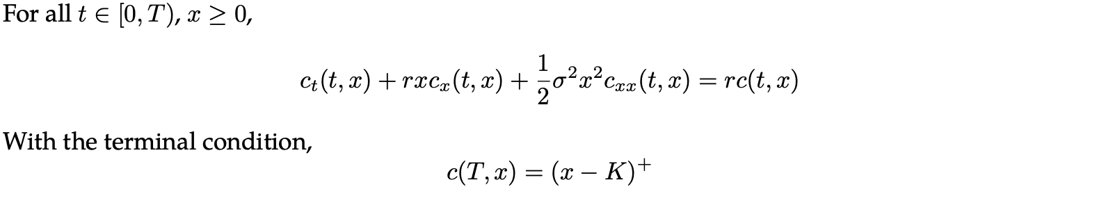
The goal is to provide an explaination of this famous PDE by using intuition, some notions of Stochastic Calculus and one of the main principles of Finance: replication.

Why does the PDE need to be studied ? Simply because the well-known expressions of Black-Scholes-Merton model are actually the solutions of this PDE. These expressions will be studied and explained in Part II.

Key assumptions

Black-Scholes-Merton model is not only famous for providing famous expressions to price derivatives but also for making genuine simple assumptions.

First and foremost, Black-Scholes-Merton model assumes that there are no commissions nor transactions costs. This means that there are no fees for buying and selling options and stocks. Moreover, the market is perfectly liquid: it is possible to purchase or sell any amount of stocks or options at any given time.

Afterwards, the Black-Scholes-Merton model only considers European-style options which can only be exercised on the expiration date whereas American-style options can be exercised at any time during the life of the option. This makes American options more valuable as they display a greater flexibility.

Volatility is a statistical measure of the dispersion of returns for a given security. In the securities markets, volatility is often associated with big swings in either direction. The volatility is assumed to be constant.

Similarly, the Black-Scholes-Merton model uses the risk-free rate to represent constant interest rates.

A log-normal distribution

Finally, the model assumes that returns on the underlying stock are log-normally distributed. This means the stock is modeled by a geometric Brownian motion. The asset price S_t has instantaneous mean rate of return α and volatility σ. Here are the dynamics of the stock under Black-Scholes-Merton model:

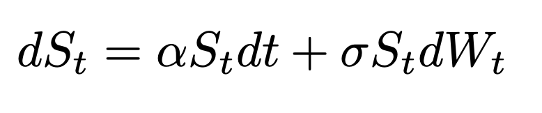
where dt represents the variation of time and it is often referred as the drift term and W_t is a Brownian motion (or Wiener process) which means that it is a stochastic (random) process with normally independent distributed increments with a normal distribution N(0,√(Δ_t)). In other words, the volatility combined with a Brownian motion represents the uncertainty or the unexpected change that might occur in the variation of the stock, dS_t.

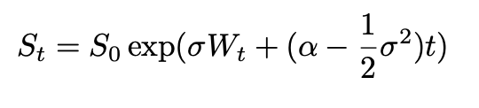
In the case of constant volatility, we can write:

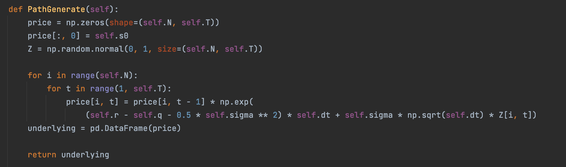
In terms of implementation, this is how different trajectories of a geometric Brownian motion can be generated:

Later, we will see which assumptions seem reasonable and which ones spawn serious limitations to the model. For now, what needs to be kept in mind is the following: constant interest rate and constant volatility.

Few notions of Finance and Stochastic Calculus

In order to complete the explaination of the PDE, there are few notions that are needed. First of all, the value of one dollar today is not the same as the value of one dollar dollar tomorrow: this is discounting. This is why it makes more sense to analyze the differential of the discounted portfolio value. Continuous compounding, with e^-rt, will be considered.

Secondly, another essential notion of Finance is needed to carry the explaination: replication. Let’s denote X, an arbitrary contingent claim (an arbitrary derivative). Replication means that one can form a trading strategy such that the terminal value of this portfolio matches the payoff of X in all states.

At last, what needs to be understood is that the analysis is made with random processes. Therefore, there is a difference between taking the derivative of a deterministic function and a stochastic process:

Deterministic functions	Stochastic processes

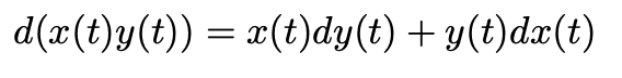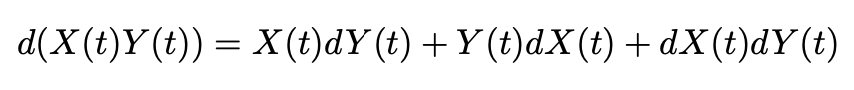This leads to several differences in the computations as Itô-Doeblin formulas need to be used. The goal is not to make a course of Stochastic Calculus, so the expression needed for an Itô process will be assumed and can be written as followed:

Where f_t is the first-order partial derivative with respect to the time variable (t), f_x is the first-order partial derivative with respect to the stock price x and f_xx is the second-order partial derivative with respect to x.

A popular Partial Differential Equation

Portfolio value

Let’s denote V_t, the value of the portfolio at each time t.

Let’s define the investing context by considering an investor holding Δ(t) shares of stock. The remainder of the portfolio value is invested in the money market account with rate r.

Thus, the differential dV_t, of the investor’s portfolio value comes from the capital gain on the stock position and the interest rate earnings. Therefore, we have:

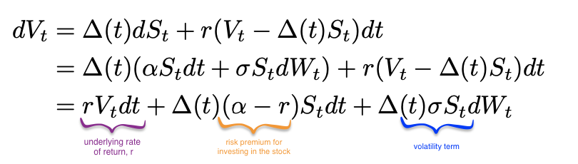
Steps to get the PDE

The goal is to use the replication property. To do so, we need to understand the variations of the discounted portfolio value as well as the variations of the discounted call price which is our contingent claim here.

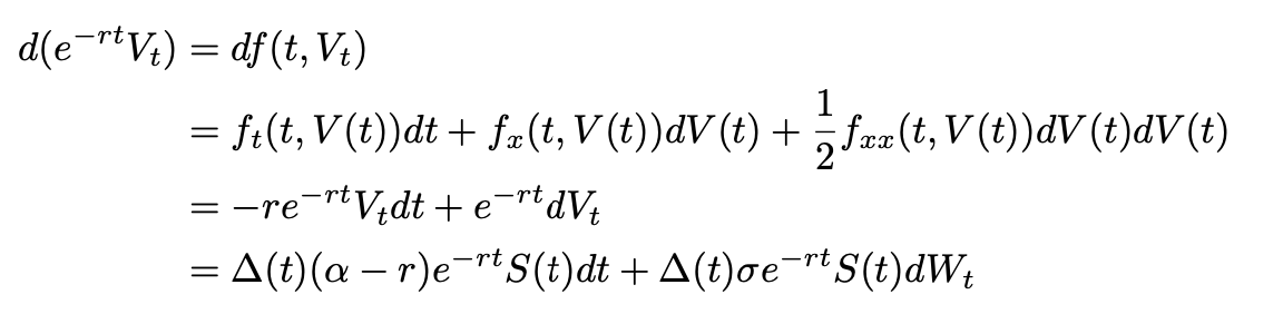
First, let’s apply this formula to the discounted portfolio value using: f(t,x)=e^-rtx. This leads to:

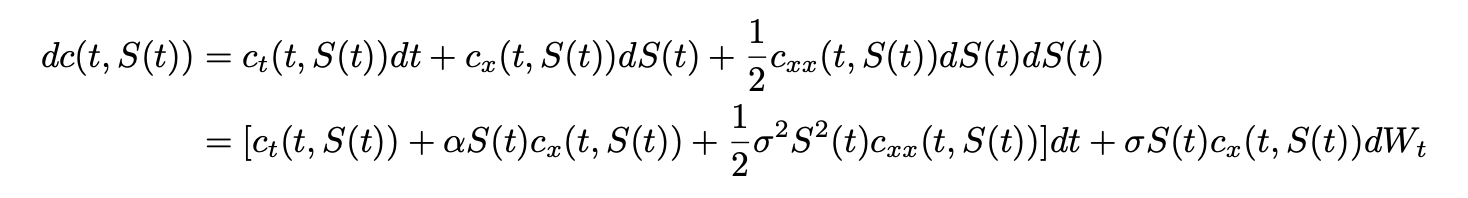
Then, let’s denote c(t,x), the value of the call at time t if the stock price at that time is S(t)=x. Let’s compute the differential of c(t,S(t)):

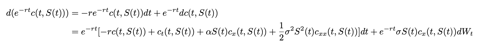
Let’s apply Itô-Doeblin formula to discounted option price.

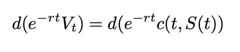
Now, the only thing that is required is to use the replication principle. A hedging portfolio starts with some initial capital V₀ and invests in the stock and the banking account in order to match V_t at each time t with c(t,S(t)). To ensure this condition, the previous equations need to be equated such that for all t between [0,T]:

Obtaining the PDE

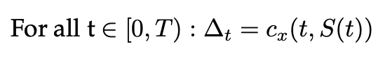
Subsequently, two key equations can be obtained. The first one is the delta-hedging rule. Indeed, if the dW_t terms are equated, we get:

Finally, by equating the dt terms, the Black-Scholes-Merton partial differential equation appears as followed:

Final thoughts

This article aimed to provide an explaination about the PDE describing Black-Scholes-Merton model and a way to obtain it. That equation can be generalized especially when the underlying asset is a geometric Brownian motion: this can be explained thanks to Feynman-Kac theorem.

What’s next ?

Now that we know how to obtain the PDE of Black-Scholes-Merton model, a continuous function c(t,x) that is solution to the PDE must be found. As a result, the well-known expressions of the model will be reviewed and detailed. The limitations of Black-Scholes-Merton will also be discussed.

Credits: Photo by Jeswin Thomas on Unsplash

Article précédent

Article suivant