-
 contact@diggers-consulting.com
  01 73 28 29 65
 LinkedIn

Motivation
The goal of this article is to present the well-known expressions of Black-Scholes-Merton model. Indeed, unlike other models, Black and Scholes originally managed to obtain closed-form expressions for options, Greeks and other derivatives with simple assumptions. These terms will be re-explained later.
These expressions that will be presented in this article can be derived from the PDE that we proved on the previous article that you can find here: https://diggers-consulting.com/finance-de-marche/from-math-to-python-black-scholes-merton-model
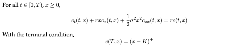
As a reminder, here is the Black-Scholes-Merton model PDE:
Closed-form expressions
First and foremost, Black-Scholes-Merton model provides expressions for call and put options. You can find a refresher about those two financial contracts on the first article of the series: https://diggers-consulting.com/finance-de-marche/from-math-to-python-financial-models.
Here are the expressions under BSM model:
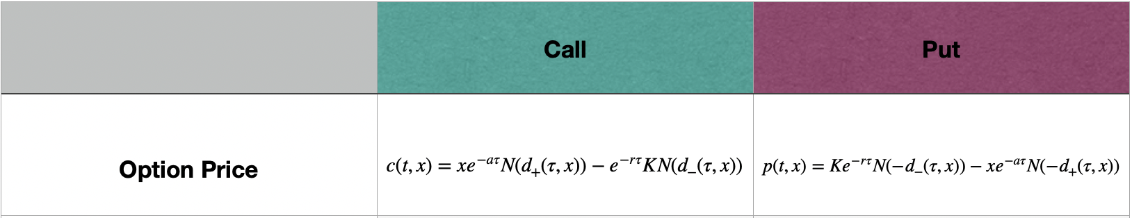
The variable x is the stock price, K is the strike price, r is the risk-free rate, a is the dividend yield and N normal distribution.
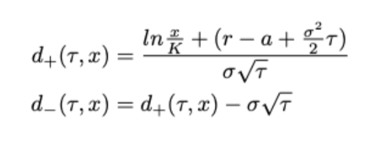
Also, we have:
The last section aims to prove that the call expression presented above is indeed a solution of the partial differential equation. It is quite a technical proof that requires some mathematical background. Therefore, it is not the most essential part of this article, and you can see it as a bonus !
Practical example
A concrete example will give the reader a clear idea of the notion of pricing and the use of those expressions.
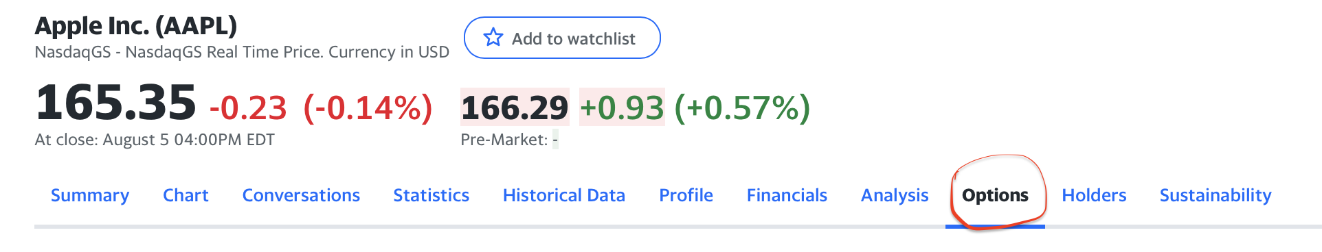
For instance, let’s consider Apple stock (AAPL). On the 8th of August 2022, imagine an investor wants to buy 100 shares of a call option. The current price of the stock is SAAPL= 166$. The investor wants a short-term maturity (September 2nd 2022) and a strike price, K=170$.
First, we can check what is the quote (meaning the the real-market price) on Yahoo Finance. If you go on AAPL ticker, you can find all the details you need about the stock. We are interested in the price of a call option:
Then, we just need to look for our financial instrument:
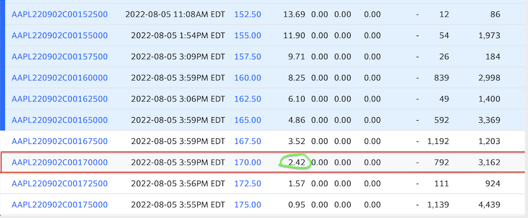
At last, we can compare this price with the one can be obtained for with Black-Scholes-Merton model. A risk-free rate of 2%, an implied volatility of 22% and τ = 20/250 are the parameters considered. The price obtained is equal to 2.46 which is actually pretty close from the quote provided.
The Greeks
Obtaining the price of an option is a good first step, but then it is important to be able to hedge any positions on this contract. There are different ways to hedge but here the focus has been realized on different metrics called The Greeks.
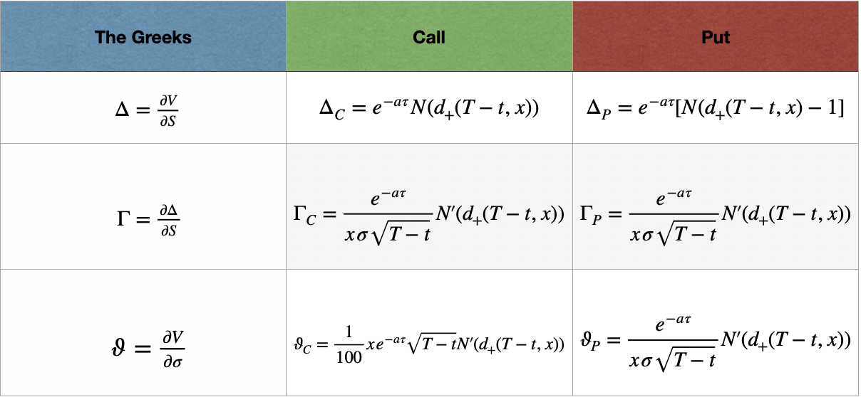
According to Investopedia, the variables that are used to assess risk in the options market are commonly referred to as The Greeks. The most common Greeks used include the Delta, Gamma and Vega, which are the first partial derivatives of the options pricing model. Let’s recall their expression:
- Delta, represents he change in the value of an option in relation to the movement in the market price of the underlying asset.
- Gamma, is the rate of change between an option’s delta and the underlying asset’s price.
- Vega, represents the rate of change between an option’s value and the underlying asset’s implied volatility.
Let’s take back the previous example to genuinely understand the relevance of Greeks for hedging purposes. The Greeks can be easily computed. For example, in this example, we have: Δ = 0,36. In order to be Delta-neutral, the investor needs to buy 36 additional shares.
Link with the library
Black-Scholes-Merton model is always a good way to start a pricing library as it gives a good first indication of where stock price stands.
The combination of Monte-Carlo Methods and analytical expressions such as those provided by BSM model is a real strength of our library. The main reason is it enables to verify that the functions are well-implemented. It also gives an interesting dilemma between time and accuracy: some methods are faster but less accurate (analytical) and vice-versa.
Limitations of the model
Black-Scholes-Merton model is based on several assumptions. Among them, some are reasonable. Indeed, assuming the market perfectly liquid or modeling the stock with a log-normal distribution (Geometric Brownian Motion) are far from being bad approximations for a financial model.
However, this model only enables to price European-style options which is a serious drawback as most of the options traded on the market are American-style options. In the Black-Scholes world, there are no taxes nor fees on transactions which is not ideal.
But more importantly, the key limitations of this model are the ones made on interest rates and volatility. Both are assumed to be constant which is far from capturing the reality.
Volatility
When approaching the question of volatility, there is a phenomenon that needs to be considered: the volatility smile.
The smile shows that the options that are furthest in the money (ITM) or out of the money (OTM) have the highest implied volatility. On the other hand, options with the lowest implied volatility have strike prices at the money (ATM) or near the money.
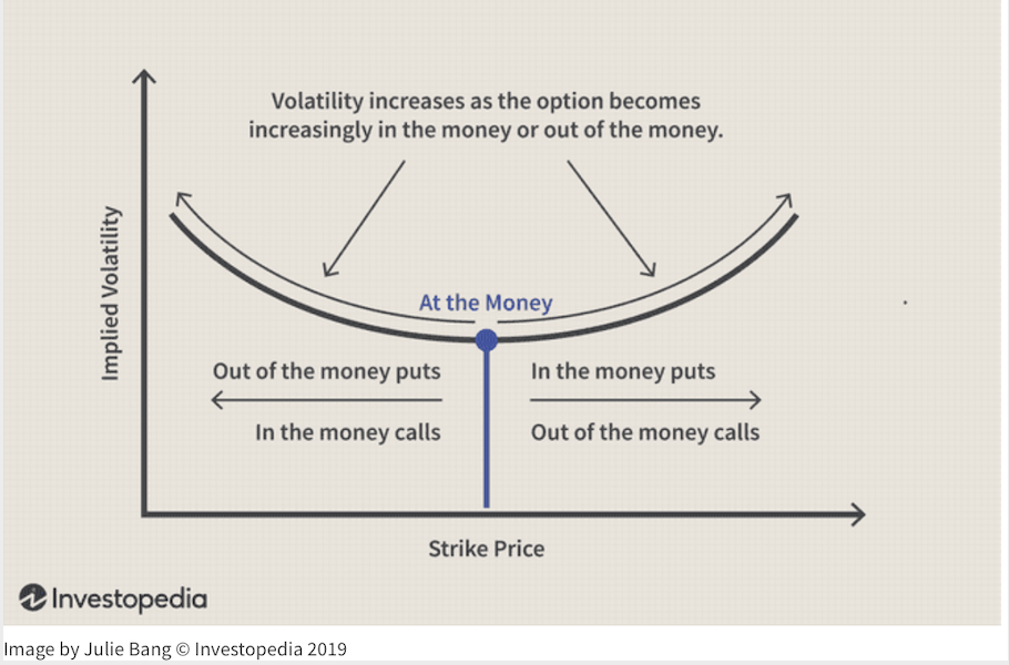
There is a real debate among traders about which volatility should be considered for Black-Scholes-Merton model. Indeed, the volatility smile is not predicted by the Black-Scholes-Merton model as the model predicts that the implied volatility curve is flat when plotted against varying strike prices.
Based on the model, it would be expected that the implied volatility would be the same for all options expiring on the same date with the same underlying asset, regardless of the strike price. Yet, in the real world, it is not the case.
Therefore, some would say that the historical volatility should be considered as it is unique. Nonetheless, it gives poor result for options with a long expiration.
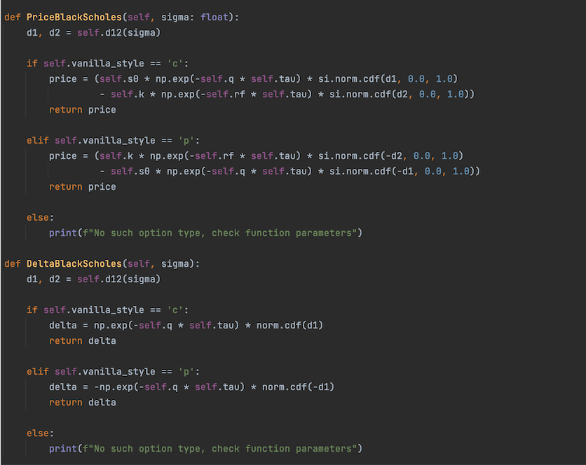
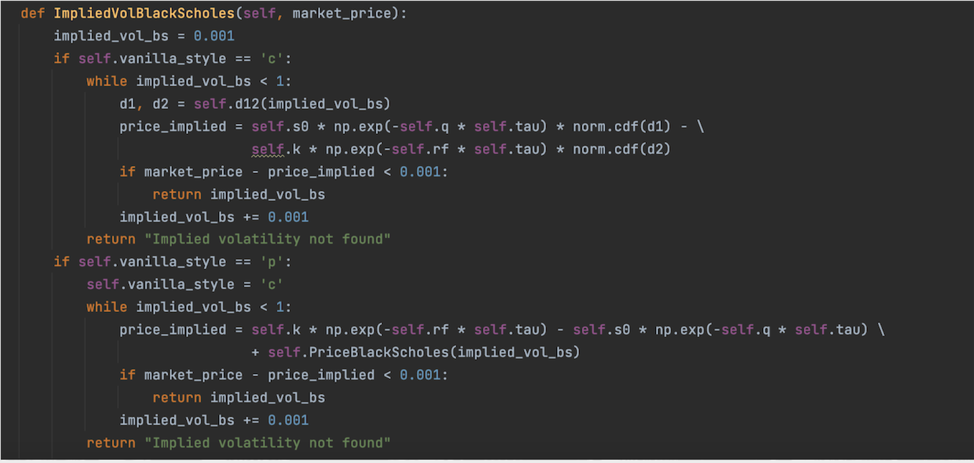
On the other hand, implied volatility can be computed easily with Black-Scholes-Merton model even thought it may not be relevant. Here is a function of our library (BlackScholesAnalytics class) that enables to obtain it:
Interest Rates
Obviously, the Black-Scholes-Merton model gives a bad representation of interest rates as it assumes them constant. The concept of « risk-free » does not exist in real life even though the 10Y Government yield could be the closest rate of this concept.
There are different ways to model interest rates. In the library, the main focus has been made on Vasicek model and its improved version: Hull-White model.
What’s next ?
This article on Black-Scholes-Merton model presented the well-known expressions that can be encountered. It showed that this model gives a good first approximation. Nevertheless, it also highlighted the volatility as a key parameter in options pricing.
Thus, volatility and the issues spawned by this parameter need to be handled. The next article will be on stochastic volatility model. This means that the volatility is assumed to be random and therefore, it displays its own dynamics. To do so, we will study Heston model !
Annex
How to get the call option price under Black-Scholes-Merton model ? Change of probability measure !
Previously, in this article, the expressions for call and put options have been presented. Making few computations, it is easy to see that there are indeed solutions of the Black-Scholes-Merton PDE. But, how can we manage to obtain these expressions ? Where do they come from ?
This is the goal of this section which is quite technical and maybe more adapted for people working or interested in Quantitative Finance.
Martingales theory
Martingale theory is key to understand the overall proof of the call expression under Black-Scholes-Merton model. However, a whole course can be made on this notion. Therefore, in summary, a martingale is a sequence of random variables for which at time t, the conditional expectation of the next value in the sequence is equal to the present value, regardless of all prior values.
More details can be found on the following link: https://people.maths.bris.ac.uk/~mb13434/mart_thy_notes.pdf
Risk-Neutral Pricing formula
The goal is not to prove the continuous-time risk-neutral pricing formula but rather to use it. Still, for those interested, let’s recall the important steps that enable to obtain this essential formula.
First of all, a discount process, D(t), must be introduced such that: dD(t) = -R(t)D(t)dt.
Then, the differential of the discounted stock price process can be written as:
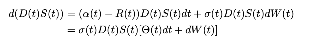
Thanks to Girsanov’s Theorem, the probability measure P-tilde can be introduced such that we may rewrite:
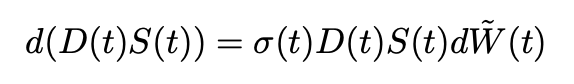
The measure define in Girsanov’s theorem is the risk-neutral measure because it is equivalent to the original measure P and it renders the discounted stock price D(t)S(t) into a martingale.
Therefore, we have:
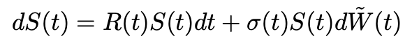
In continuous-time, the change from the actual measure P to the risk-neutral measure P-tilde changes the mean rate of return of the stock but not the volatility.
Afterwards, the value of the portfolio process under the Risk-Neutral Measure must be investigated.
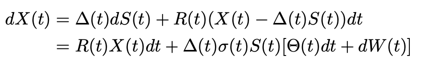
Using Itô’s product rule, we get:

Hence, the discounted value of the portfolio is a martingale under the risk-neutral probability measure.
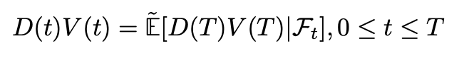
This means that:

where V is the payoff of the derivative security.
This is the the continuous-time risk-neutral pricing formula:
Call expression under BSM model
Consider a stock, modeled as a generalized Brownian motion, that pays dividends over time at a rate A(t) per unit time. Here A(t) is a non-negative process. Dividends paid by a stock reduce its value. Thus, the model for the stock price can be written as followed:
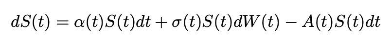
With constant coefficients σ, r, and a, this leads to:
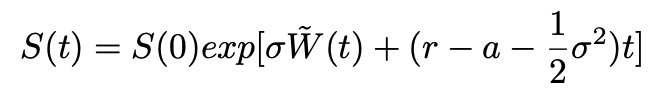
According to the risk-neutral pricing formula, the price at time t of a European call expiring at time T with strike K is:
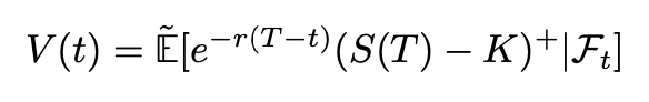
We can compute c(t,x) using the Independence Lemma. Then, the only thing remaining is computations !
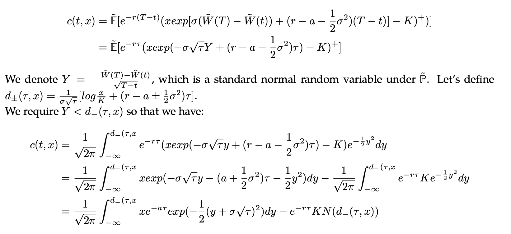
At last, we make the change of variable z = y+σ√τ in the integral, which leads us to the following formula:
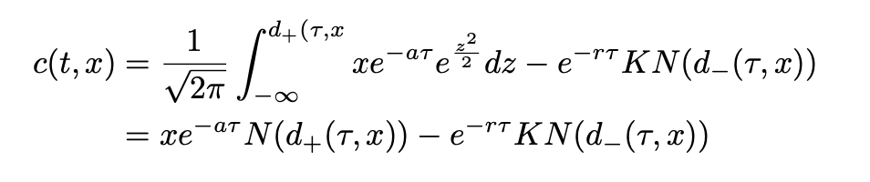
The expression for a put option can be obtained by applying the same method or by using Put-call parity.
Credits: Photo by Tyler Prahm on Unsplash
| Article précédent | Article suivant |